
While learning more about electron beam lithography, I had one practical question.
Suppose someone gives me a GDSII file and asks me to write the pattern using EBL.
The pattern is already designed. The dimensions are already there in the GDS file.
But one thing is still missing.
How do I know what dose I should use?
Can I just look at the GDS file and decide that this pattern needs 250 µC/cm² or 300 µC/cm²?
Or do I have to write the pattern with different doses first and check which one gives the result I actually want?
This is what I wanted to understand.
First, What Does the GDSII File Give Us?
When we load a GDSII file, we already have the pattern geometry.
For example, the file can contain:
- lines
- rectangles
- circles or polygons
- different layers
- arrays
- alignment marks
- nanoscale structures
Suppose I open a GDS file and there is a line designed to be:
100 nm wide
The GDS tells me:
This is the geometry I want to fabricate.
But the GDS file itself does not automatically tell me:
Use exactly 300 µC/cm² and you will get a perfect 100 nm line.
This was an important difference for me to understand.
CAD/GDS tells us what we want to write.
The exposure process decides how we are going to write it.
Can We Decide the Dose Just From the Pattern Size?
At first I thought maybe the pattern dimension would directly tell us the required dose.
For example:
100 nm line = one dose
50 nm line = another dose
But it is not that simple.
The required exposure depends on the complete process.
For example, we need to know things like:
What resist are we using?
How thick is the resist?
What acceleration voltage are we using?
What is the substrate?
What development condition are we using?
Is the pattern isolated or very dense?
So two people can have similar GDS patterns but use different process conditions and may not end up using exactly the same dose.
That means there is no universal rule like:
100 nm pattern = 300 µC/cm²
We need a starting point, but then we need to check the actual result.
So Where Do We Get the Starting Dose?
We don’t normally start completely from zero.
If the same resist and similar process have already been used before, there may already be a known starting dose or process recipe.
The resist information, previous experiments, published work or experience with the process can also help us choose a reasonable starting range.
Let’s take a simple example.
Suppose from previous information I think that a useful dose may be somewhere around:
300 µC/cm²
I could expose the pattern only at 300 µC/cm².
But if this is a new process or an important feature, how do I know that 300 is actually the best condition?
This is where a dose test becomes useful.
Writing the Same Pattern With Different Doses
Instead of writing only one pattern at one dose, I can make several copies of the same test pattern.
For example:
| Pattern | Dose |
|---|---|
| A | 250 µC/cm² |
| B | 275 µC/cm² |
| C | 300 µC/cm² |
| D | 325 µC/cm² |
| E | 350 µC/cm² |
Now I have the same basic pattern, but each copy receives a different nominal dose.
This is important because I am trying to change mainly one thing:
the exposure dose.
After exposure, I develop the resist using controlled development conditions.
Then I can compare what happened.
What Am I Looking For After Development?
Suppose my GDS contains a target 100 nm line.
After exposure and development, I inspect the test patterns with suitable metrology, for example SEM when appropriate.
Maybe I see something like this:
250 µC/cm²
Pattern did not develop as expected.
275 µC/cm²
Pattern looks better, but the dimensions are still not what I want.
300 µC/cm²
Pattern is close to the intended result.
325 µC/cm²
The feature starts changing more than I want.
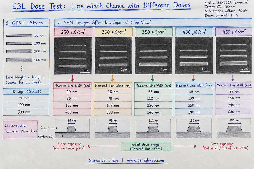
350 µC/cm²
The result is clearly different from the target.
These numbers are only an example to understand the method. They do not mean that 300 µC/cm² is the correct dose for every 100 nm pattern.
Also, whether increasing dose makes a particular measured feature appear wider, narrower, more cleared, or more filled depends on the resist tone and what geometry we are measuring.
The important point is the comparison.
I have:
Designed pattern
vs.
Actual developed pattern
Now I can see which exposure condition gives the result closest to what I need.
Dose Is Not the Same as Beam Current
This is another thing that confused me when I started connecting these topics.
Suppose I decide that my required dose is:
300 µC/cm²
Then I select a beam current.
Are dose and beam current the same thing?
No.
Dose tells me how much charge I want to deliver per exposed area.
Beam current tells me how quickly the electron beam is delivering charge.
The basic relation is:
So if I use a lower current, I generally need more beam-on time to deliver the same charge.
If I use a higher current, I can deliver that charge faster.
This connects with my previous topic about beam current, aperture and spot size.
But choosing a higher current just to make exposure faster is not always the answer, because the beam condition also has to be suitable for the feature we want to write.
What If My GDS Contains Different Types of Patterns?
Now there is another problem.
A real GDS file may not contain only one simple line.
It may have:
isolated lines
dense lines
small gaps
large exposed areas
corners
different feature sizes
Now I cannot always assume that every part of the pattern will behave exactly the same just because I assigned the same nominal dose.
Electron scattering and the proximity effect can make dense and isolated structures behave differently.
This is why dose optimization can become more complicated for real patterns.
For a simple test, trying several doses may be enough to find a useful process window.
For more complicated nanoscale patterns, we may also need to think about proximity-effect correction and local dose modification.
I will keep that as a separate topic because otherwise this article will become too long.
What I Understood
Before thinking about this, I had a simple picture in my mind:
Load GDS → select dose → write pattern.
But now I understand there is an important step between the design and the final process.
For a new pattern, my thinking should be more like:
GDSII pattern
↓
Understand the pattern and process conditions
↓
Choose a reasonable starting dose/range
↓
Create a dose test
↓
Expose
↓
Develop
↓
Inspect and measure
↓
Compare with the intended geometry
↓
Adjust if necessary
↓
Establish the process condition
The GDS file gives us the target geometry.
The EBL exposure parameters help us reproduce that geometry in the resist.
And the experimental result tells us whether our process is actually giving us what we designed.
One More Thing I Learned
There is also a bigger picture here.
Suppose the GDS pattern is part of a transistor.
The EBL dose test is not directly telling me how much electrical current that transistor will eventually carry.
At this stage I am asking:
Did I fabricate the nanoscale geometry correctly?
After the complete device is fabricated, the researcher can electrically test the transistor and compare its real performance with the original device design or simulation.
So these are different steps:
Device design/simulation
↓
GDS layout
↓
EBL process optimization
↓
Fabrication
↓
Physical inspection
↓
Electrical testing
This helped me understand where EBL actually fits into the much bigger semiconductor-development process.
Conclusion
Having a GDSII file does not mean that every EBL parameter is already decided.
The GDS tells us what pattern we want.
But we still need to determine how to expose that pattern under our actual resist, substrate and beam conditions.
For a new process, one practical approach is to start from previous knowledge, choose a reasonable dose range, expose several test patterns, develop them under controlled conditions and compare the results.
For me, the biggest lesson was simple:
We don’t choose an EBL dose only because a number looks correct. We expose, develop, measure and learn from the actual pattern.
And that is where a CAD drawing starts becoming a real nanoscale structure.

Leave a Reply